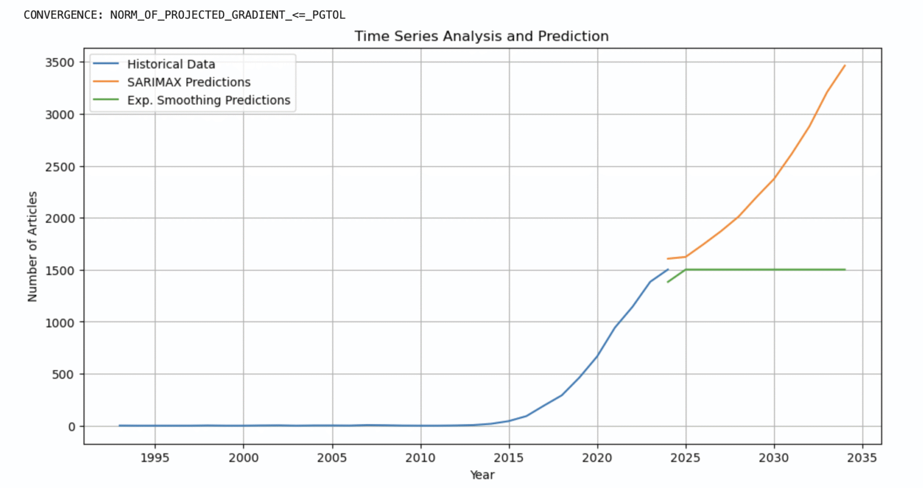
The autoregressive (A.R.) model is a specific time series model that predicts future values based on historical ones. Its simplicity in implementation and comprehension makes A.R. models a common choice for forecasting time series data. A noteworthy enhancement to the traditional ARIMA (Auto-Regressive Integrated Moving Average) model is the Seasonal Autoregressive Integrated Moving Average with Exogenous Regressors (SARIMAX) model, which considers seasonality and external influences (Hewamalage et. al., 2023). This versatile model allows for the inclusion of external variables or regressors, employs differencing for data stabilisation, and manages both autoregressive (A.R.) and moving average (M.A.) components. SARIMAX proves particularly beneficial when dealing with time-dependent data that reveal recurring patterns over specific intervals (Mulla et al., 2024).
1.1 SARIMAX Model:
The ARIMA model consists of three main components. First, the AR stands for Auto Regressive, which uses earlier values of the variable to describe its behaviour (Hwarng 2001), and this is indicated by the Auto Regressive order p. Next, I represents Integrated, signified by d, which refers to the differencing order. Finally, we have the Moving Average model, which captures the variable’s behaviour based on random errors from previous periods (Hwarng 2001), represented by the Moving Average Order q. The ARIMA model is applied to stationary datasets; however, if there is seasonality in the dataset, the Seasonal ARIMA, or SARIMA model, may be used instead. This model is expressed as (p,d,q) (P, D, Q)s, where P, D, and Q represent the seasonal orders analogous to p,d, and q in the ARIMA model, and s signifies the seasonality. There’s also an enhanced version known as SARIMAX (Seasonal Auto-Regressive Integrated Moving Average with eXogenous factors), Which incorporates external influences alongside the model’s autoregressive and moving average elements (Hyndman & Athanasopoulos, 2018). Therefore, SARIMAX can be viewed as a seasonal model that is similar to both SARIMA and Auto ARIMA. Mathematically, this model is represented as,
1.2. Exponential Smoothing Model:
For univariate data, exponential smoothing is a time series forecasting technique. A model with a prediction that is a weighted linear sum of recent historical data or lags is developed using time series techniques, such as the Box-Jenkins ARIMA family of approaches. While the model explicitly utilised an exponentially decreasing weight for earlier observations, exponential smoothing forecasting approaches are similar in that a prediction is a weighted sum of past observations.
1.2.1 Simple Exponential Smoothing:
A time series forecasting technique for univariate data without a trend or seasonality is termed Simple Exponential Smoothing, or S.E.S. for short. It is also known as Single Exponential Smoothing. It needs one parameter known as alpha (α), sometimes called the smoothing coefficient or factor.
 (Hyndman & Athanasopoulos, 2018). This parameter controls the exponential decay rate influenced by the observations from earlier time steps. Usually, alpha is assigned to a number between 0 and 1. Smaller numbers show that more of the past is considered when producing predictions, but large values show that the model focuses mainly on the most recent past observations.
1.2.2 Double Exponential Smoothing:
A variation of exponential smoothing that specifically supports trends in the univariate time series is called double exponential smoothing. The decay of the influence of the trend change is regulated by a second smoothing factor called beta (β), which is added to the alpha parameter that controls the smoothing factor for the Level. Depending on whether a trend is linear or exponential, the approach can accommodate both additive and multiplicative changes. Traditionally, double exponential smoothing with an additive trend is known as Holt’s linear trend model, created after Charles Holt, the method’s creator (Holt, 1957). Double Exponential Smoothing with a linear trend has an additive trend. Double exponential smoothing with an exponential trend is known as multiplicative trending.
1.2.3 Triple Exponential Smoothing:
A variation of exponential smoothing that specifically supports seasonality in the univariate time series is called triple exponential smoothing. Because Charles Holt (1957) and Peter Winters (1960) were two of the method’s contributors, the technique is also occasionally called Holt-Winters Exponential Smoothing (Winters, 1960; Holt, 2004). A new parameter called gamma (γ) is added to the alpha and beta smoothing parameters to control the influence on the seasonal part. Like the trend, the seasonality can be represented as a linear or exponential change in the seasonality using either an additive or multiplicative approach. Triple Exponential Smoothing with a linear seasonality is Additive Seasonality. Triple exponential smoothing with exponential seasonality is known as multiplicative seasonality.
The most sophisticated kind of exponential smoothing is called triple exponential smoothing, and with the proper setup, it can additionally develop simple and double exponential smoothing models.
References:
Hyndman, R.J., & Athanasopoulos, G. (2018), Forecasting: principles and practice, 2nd edition. Melbourne, Australia.
Winters, P. R. (1960), “Forecasting Sales by Exponentially Weighted Moving Averages”, Management Science, Vol. 6 No. 3, pp. 324-342.
Hewamalage, H., Ackermann, K. and Bergmeir, C. (2023), “Forecast evaluation for data scientists: common pitfalls and best practices”, Data Mining and Knowledge Discovery, Vol. 37 No. 2, pp. 788-832.
Mulla, S., Pande, C. B. and Singh, S. K. (2024), “Times Series Forecasting of Monthly Rainfall using Seasonal Auto Regressive Integrated Moving Average with EXogenous Variables (SARIMAX) Model”, Water Resources Management, Vol. 38 No. 6, pp. 1825-1846.
Holt, C. C. (1957), “Forecasting trends and seasonals by exponentially weighted averages”, O.N.R. Memorandum, Vol. 52.
Hwarng, H. B. (2001), “Insights into neural-network forecasting of time series corresponding to ARMA (p; q) structures”, Omega, pp. 273-289.


